Visualizing the prevalence of diabetes in six European countries, 1990-2017

This is a quick demonstration of diabetes prevalence in six European countries. The data are from the the Institute of Health Metrics and Evaluation (IHME).

A step by-step guide on how to improve a simple scatter plot

My R version

• See below

version

               _                           
platform       x86_64-w64-mingw32          
arch           x86_64                      
os             mingw32                     
system         x86_64, mingw32             
status                                     
major          4                           
minor          1.3                         
year           2022                        
month          03                          
day            10                          
svn rev        81868                       
language       R                           
version.string R version 4.1.3 (2022-03-10)
nickname       One Push-Up                 

Required packages

#If you don't have any of these packages install them using install.packages("pakage)
library(readr) #to read csv file
library(dplyr) #for data manipulaion 
library(ggplot2) # for awesome plotting
library(gganimate) #for animating ggplot objects
library(scales) # for customizing axis 
library(lattice) #for enhancing graphics
library(directlabels) #for directly labeling!
library(transformr)

Load the data and have a closer look

# The data is for all countries included in GBD studies
diabetes <- read_csv("Eurodiabetes.csv") 
dim(diabetes) #980 observations and 9 variables. 

[1] 980   9

str(diabetes) 

spc_tbl_ [980 x 9] (S3: spec_tbl_df/tbl_df/tbl/data.frame)
 $ Location                : chr [1:980] "Australia" "Australia" "Australia" "Australia" ...
 $ Year                    : num [1:980] 1990 1991 1992 1993 1994 ...
 $ Age                     : chr [1:980] "All ages" "All ages" "All ages" "All ages" ...
 $ Sex                     : chr [1:980] "Both" "Both" "Both" "Both" ...
 $ Cause of death or injury: chr [1:980] "Diabetes mellitus" "Diabetes mellitus" "Diabetes mellitus" "Diabetes mellitus" ...
 $ Measure                 : chr [1:980] "Percent of total prevalent cases" "Percent of total prevalent cases" "Percent of total prevalent cases" "Percent of total prevalent cases" ...
 $ Value                   : num [1:980] 0.0503 0.0497 0.0492 0.0488 0.0486 ...
 $ Lower bound             : num [1:980] 0.0546 0.054 0.0532 0.0528 0.0526 ...
 $ Upper bound             : num [1:980] 0.0462 0.0459 0.0456 0.0453 0.045 ...
 - attr(*, "spec")=
  .. cols(
  ..   Location = col_character(),
  ..   Year = col_double(),
  ..   Age = col_character(),
  ..   Sex = col_character(),
  ..   `Cause of death or injury` = col_character(),
  ..   Measure = col_character(),
  ..   Value = col_double(),
  ..   `Lower bound` = col_double(),
  ..   `Upper bound` = col_double()
  .. )
 - attr(*, "problems")=<externalptr> 

Let’s choose only 5 European countries with high diabetes prevalence

ger_au_ch <- diabetes %>% 
  filter(Location %in% c("Austria", "Germany", "Switzerland", "Denmark", "Portugal", "Finland")) 
ger_au_ch <- na.omit(ger_au_ch) #Remove missing values
ger_au_ch$Prev <- ger_au_ch$Value*100 #Prevalence in percent. 
str(ger_au_ch) #structure of the data, variable types

tibble [168 x 10] (S3: tbl_df/tbl/data.frame)
 $ Location                : chr [1:168] "Austria" "Austria" "Austria" "Austria" ...
 $ Year                    : num [1:168] 1990 1991 1992 1993 1994 ...
 $ Age                     : chr [1:168] "All ages" "All ages" "All ages" "All ages" ...
 $ Sex                     : chr [1:168] "Both" "Both" "Both" "Both" ...
 $ Cause of death or injury: chr [1:168] "Diabetes mellitus" "Diabetes mellitus" "Diabetes mellitus" "Diabetes mellitus" ...
 $ Measure                 : chr [1:168] "Percent of total prevalent cases" "Percent of total prevalent cases" "Percent of total prevalent cases" "Percent of total prevalent cases" ...
 $ Value                   : num [1:168] 0.0562 0.0579 0.0597 0.0614 0.0631 ...
 $ Lower bound             : num [1:168] 0.061 0.0627 0.0646 0.0664 0.0683 ...
 $ Upper bound             : num [1:168] 0.0519 0.0538 0.0555 0.0572 0.0588 ...
 $ Prev                    : num [1:168] 5.62 5.79 5.97 6.14 6.31 ...

dim(ger_au_ch) #168 rows, 10 columns 

[1] 168  10

is.factor(ger_au_ch$Year) #check if Year is saved as factor variable

[1] FALSE

ger_au_ch$yearfactor <- factor(ger_au_ch$Year) #convert it to factor and save it as Yearfactor

ger_au_ch$Yearnumeric <- as.numeric(ger_au_ch$Year) #change it to numeric and save it as Year Numeric

Basic plots

Since we already have everything we need for plotting, we can start using ggplot2

plot1 <- ggplot(ger_au_ch, aes(x=Yearnumeric, y=Prev, col=Location)) + 
  geom_line() + geom_point() + xlab("Year") +
  ylab("Prevalence of diabetes in %") 
plot1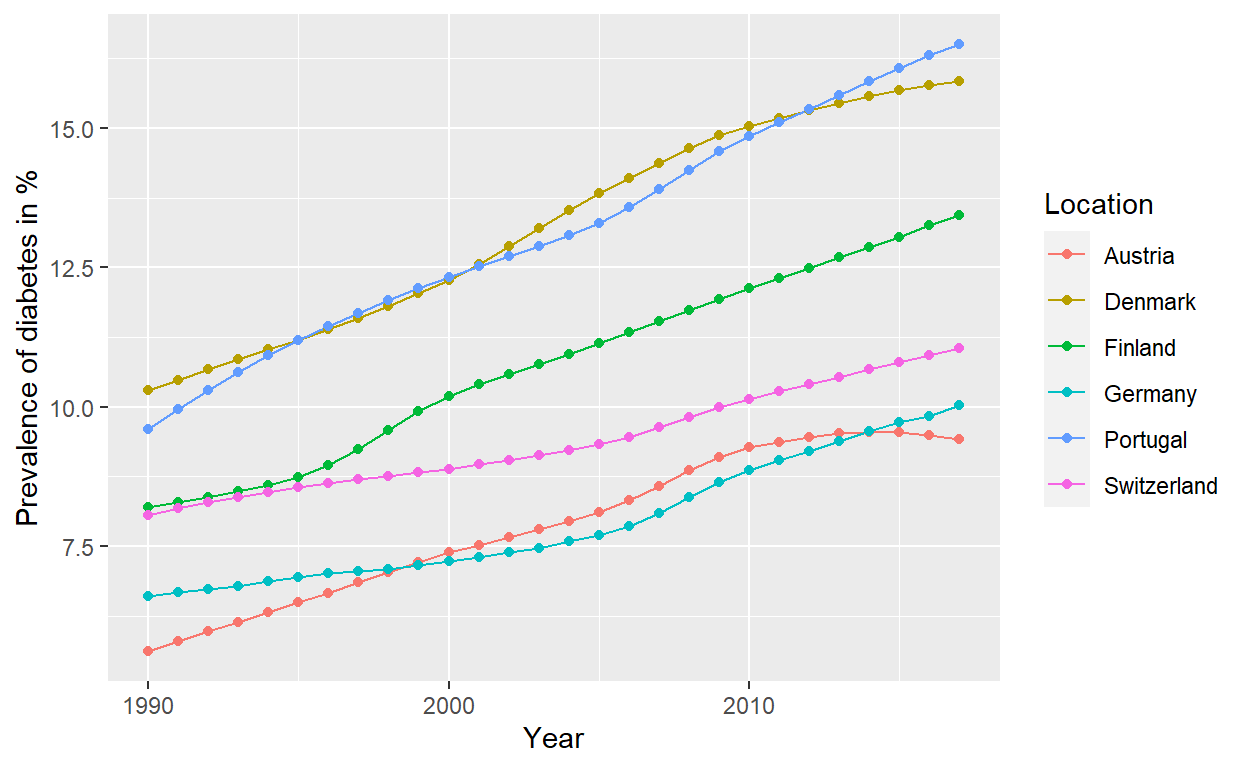

plot2 <- ggplot(ger_au_ch, aes(x=Yearnumeric, y=Prev, col=Location)) + 
  geom_line() + xlab("Year") +
  ylab("Prevalence of diabetes in %") 
plot2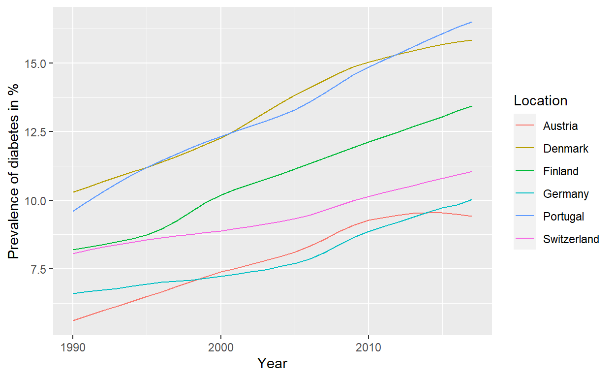

The fun part

library(gganimate)
library(directlabels)
euro_anim <- ggplot(ger_au_ch, aes(x=Yearnumeric, y=Prev, col=Location)) + 
  geom_point(size=6) + transition_time(Yearnumeric)  +
  shadow_mark()  +  
  scale_x_continuous(name ="Year",
                     breaks= c(1990,1995,2000,2005, 
                               2010, 2015, 2020)) +
  
  xlab("Year") +
  ylab("Prevalence of diabetes in %") +
  labs(col="Country") + 
  
  theme(
    axis.title.x = element_text(color = "Blue", size=15),
    axis.title.y = element_text(color = "Blue", size=15),
    axis.text.x = element_text(size = 15),
    axis.text.y = element_text(size = 15),
    
    plot.title = element_text(size=20),
    
    legend.title = element_text(size = 10),
    legend.text = element_text(size = 10),
    legend.position = "None",
    
    text = element_text(family = "Comics Sans MS")
  ) + ease_aes('cubic-in-out') +
  geom_dl(aes(label=Location),
          method=list("last.points",rot=40)) 

Use gifski_renderer to loop or no to loop the gif

• Let’s see, how it looks if we assign RUE or just T in short for loop.

animate(euro_anim, renderer = gifski_renderer(loop = T), width = 700, height = 700, duration = 15) # when you assign loop=TRUE or just T, the gif starts playing again 

• Assign loop to False or just F

  animate(euro_anim, renderer = gifski_renderer(loop = F), width = 700, height = 700, duration = 15) # when you assign loop=TRUE or just F, the gif stops looping. It only plays once. Refresh if you want to see again